With the rise of Facebook, YouTube, TikTok, and the online media economy, digital advertising is taking an ever-bigger share of the total advertising spending. As a result, tracking ad click events is very important. In this blog post, we explore how to design an ad click event aggregation system at Facebook or Google scale.
Before we dive into technical design, let’s learn about the core concepts of online advertising to better understand this topic. One core benefit of online advertising is its measurability, as quantified by real-time data.
Understanding the Problem: Real-Time Bidding and Ad Click Tracking
Digital advertising has a core process called Real-Time Bidding (RTB), in which digital advertising inventory is bought and sold. The speed of the RTB process is important as it usually occurs in less than a second.
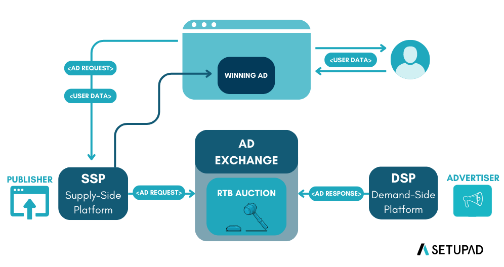
The RTB process involves several key players:
- Publisher: A website or online platform that wants to monetize its content by selling ad spaces
- Supply-Side Platform (SSP): Technology publishers use to manage and make their ad inventory available for sale
- Ad Exchange: Digital marketplace that brings together advertisers and publishers, facilitating the real-time auction process
- Demand-Side Platform (DSP): Technology that advertisers use to manage and launch their ad campaigns
- Advertiser: The company or brand that wants to display its ads online to reach its target audience
When a user visits a webpage, the available ad spaces are auctioned in real-time on the ad exchange. Advertisers’ DSPs evaluate the ad inventory and submit bids based on targeting criteria. The highest bidder wins the auction, and their ad is displayed to the user—all happening in less than a second.
📚 Want to learn more about Real-Time Bidding? Check out this comprehensive guide: What is Real-Time Bidding (RTB)?
Data accuracy is also very important. Ad click event aggregation plays a critical role in measuring the effectiveness of online advertising, which essentially impacts how much money advertisers pay. Based on the click aggregation results, campaign managers can control the budget or adjust bidding strategies, such as changing targeted audience groups, keywords, etc. The key metrics used in online advertising, including click-through rate (CTR) and conversion rate (CVR), depend on aggregated ad click data.
What is an Ad Click Aggregator?
An Ad Click Aggregator is a system that collects and aggregates data on ad clicks. It is used by advertisers to track the performance of their ads and optimize their campaigns. For our purposes, we will assume these are ads displayed on a website or app, like Facebook.
Step 1: Understand the Problem and Establish Design Scope
Functional Requirements
Core Requirements:
-
Users can click on an ad and be redirected to the advertiser’s website: When a user clicks on an ad displayed on a website or app, they should be redirected to the advertiser’s website after the click is tracked.
-
Advertisers can query ad click metrics over time with a minimum granularity of 1 minute: Advertisers should be able to query aggregated click metrics for their ads. The system must support:
- Query the number of click events for a particular ad in the last M minutes
- Query the top N most clicked ads in the past M minutes (both N and M should be configurable)
- Support data filtering by
ip,user_id, orcountryfor the above queries
Out of Scope:
- Ad targeting
- Ad serving
- Cross device tracking
- Integration with offline marketing channels
- Fraud or spam detection
- Demographic and geo profiling of users
- Conversion tracking
Non-Functional Requirements
-
Correctness: The correctness of the aggregation result is important as the data is used for RTB and ads billing. Even small discrepancies can result in significant financial impact.
-
Fault Tolerance: The system should properly handle delayed or duplicate events and be resilient to partial failures. Different components may fail independently, and the system should continue operating.
-
Scalability: The system must be scalable to support a peak of 50,000 clicks per second and handle 1 billion events per day. The system should be able to grow 30% year-over-year.
- Latency:
- End-to-end latency should be a few minutes, at most, for aggregation results (acceptable for billing and reporting purposes)
- Low latency analytics queries for advertisers (sub-second response time for querying aggregated data)
- As real-time as possible - advertisers should be able to query data as soon as possible after the click
- Idempotency: We should not count the same click multiple times. Each unique click should be counted exactly once, even if the event is processed multiple times.
Back-of-the-Envelope Estimation
Now that we’ve established our requirements, let’s understand the scale of the system. For this design in particular, the scale will have a large impact on the database design and the overall architecture.
Let’s do an estimation to understand the scale of the system and the potential challenges we will need to address:
System Scale:
- 2 million active ads in total
- 1 billion ad clicks per day
- 30% year-over-year growth rate
Note: While we list the total number of active ads for context, our primary calculations will focus on the click volume and growth rate as these directly impact our system’s performance requirements.
Traffic Estimation:
- 1 billion DAU (Daily Active Users)
- Assume on average each user clicks 1 ad per day. That’s 1 billion ad click events per day.
- Ad click QPS = 10⁹ events / 86,400 seconds in a day ≈ 10,000 QPS
- Assume peak ad click QPS is 5 times the average number. Peak QPS = 50,000 QPS.
Storage Estimation:
- Assume a single ad click event occupies 0.1 KB storage. Daily storage requirement is: 0.1 KB * 1 billion = 100 GB.
- The monthly storage requirement is about 3 TB.
Step 2: Propose High-Level Design
In this section, we discuss query API design, data model, and high-level design.
Query API Design
The purpose of the API design is to have an agreement between the client and the server. In our case, a client is the dashboard user (data scientist, product manager, advertiser, etc.) who runs queries against the aggregation service.
We only need two APIs to support the three use cases because filtering (the last requirement) can be supported by adding query parameters to the requests.
API 1: Aggregate the number of clicks of ad_id in the last M minutes
Endpoint: GET /v1/ads/{:ad_id}/aggregated_count
Request parameters:
from: Start minute (default is now minus 1 minute) -longto: End minute (default is now) -longfilter: An identifier for different filtering strategies. For example, filter = 001 filters out non-US clicks -long
Response:
ad_id: The identifier of the ad -stringcount: The aggregated count between the start and end minutes -long
API 2: Return top N most clicked ad_ids in the last M minutes
Endpoint: GET /v1/ads/popular_ads
Request parameters:
count: Top N most clicked ads -integerwindow: The aggregation window size (M) in minutes -integerfilter: An identifier for different filtering strategies -long
Response:
ad_ids: A list of the most clicked ads -array
Data Model
There are two types of data in the system: raw data and aggregated data.
Raw Data
Below shows what the raw data looks like when received from user clicks:
| ad_id | click_timestamp | user_id | ip | country | impression_id |
|---|---|---|---|---|---|
| ad001 | 2021-01-01 00:00:01 | user1 | 207.148.22.22 | USA | imp_001_abc123 |
| ad001 | 2021-01-01 00:00:02 | user1 | 207.148.22.22 | USA | imp_001_def456 |
| ad002 | 2021-01-01 00:00:02 | user2 | 209.153.56.11 | USA | imp_002_xyz789 |
Aggregated Data
Assume that ad click events are aggregated every minute. The aggregated result looks like:
| ad_id | click_minute | count |
|---|---|---|
| ad001 | 202101010000 | 5 |
| ad001 | 202101010001 | 7 |
To support ad filtering, we add an additional field called filter_id to the table:
| ad_id | click_minute | filter_id | count |
|---|---|---|---|
| ad001 | 202101010000 | 0012 | 2 |
| ad001 | 202101010000 | 0023 | 3 |
| ad001 | 202101010001 | 0012 | 1 |
| ad001 | 202101010001 | 0023 | 6 |
Raw Data vs Aggregated Data: Should We Store Both?
| Raw data only | Aggregated data only | |
|---|---|---|
| Pros | Full data set; support data filter and recalculation | Smaller data set; fast query |
| Cons | Huge data storage; slow query | Data loss. This is derived data. For example, 10 entries might be aggregated to 1 entry |
Our recommendation is to store both:
-
Raw data serves as backup data: If something goes wrong, we could use the raw data for debugging. If the aggregated data is corrupted due to a bad bug, we can recalculate the aggregated data from the raw data, after the bug is fixed. We usually don’t need to query raw data unless recalculation is needed. Old raw data could be moved to cold storage to reduce costs.
-
Aggregated data serves as active data: The data size of the raw data is huge. The large size makes querying raw data directly very inefficient. To mitigate this problem, we run read queries on aggregated data. It is tuned for query performance.
Choose the Right Database
When it comes to choosing the right database, we need to evaluate the following:
- What does the data look like? Is the data relational? Is it a document or a blob?
- Is the workflow read-heavy, write-heavy, or both?
- Is transaction support needed?
- Do the queries rely on many online analytical processing (OLAP) functions like SUM, COUNT?
For raw data:
- As shown in the back of the envelope estimation, the average write QPS is 10,000, and the peak QPS can be 50,000, so the system is write-heavy.
- Relational databases can do the job, but scaling the write can be challenging. NoSQL databases like Cassandra and InfluxDB are more suitable because they are optimized for write and time-range queries.
- Another option is to store the data in Amazon S3 using one of the columnar data formats like ORC, Parquet, or AVRO.
For aggregated data:
- It is time-series in nature and the workflow is both read and write heavy.
- The system is write-heavy because data is aggregated and written every minute by the aggregation service (2 million ads × aggregation frequency).
- It’s also read-heavy because advertisers frequently query their ad performance metrics, and dashboard systems need to display real-time analytics.
- We could use the same type of database to store both raw data and aggregated data (e.g., both in Cassandra), which simplifies operations but may not be optimal for performance. However, we recommend using specialized OLAP databases like Redshift, Snowflake, or BigQuery for aggregated data, which are specifically optimized for analytical queries and aggregations, providing much faster query performance for advertisers.
High-Level Design
In real-time big data processing, data usually flows into and out of the processing system as unbounded data streams. The aggregation service works in the same way; the input is the raw data (unbounded data streams), and the output is the aggregated results.
System Interface
For data processing questions like this one, it helps to start by defining the system’s interface. This includes clearly outlining what data the system receives and what it outputs, establishing a clear boundary of the system’s functionality. The inputs and outputs of this system are very simple, but it’s important to get these right!
Input: Ad click data from users. When a user clicks on an ad, the click event is sent directly to our server via HTTP request. Each event contains the raw data fields we defined earlier: ad_id, click_timestamp, user_id, ip, country, and impression_id (for idempotency).
Output: Ad click metrics for advertisers. This corresponds to the aggregated data structure we designed above, including click counts per minute, top clicked ads, and filtered metrics based on various criteria (using the filter_id field from our data model).
Data Flow
The data flow is the sequential series of steps we’ll cover in order to get from the inputs to our system to the outputs:
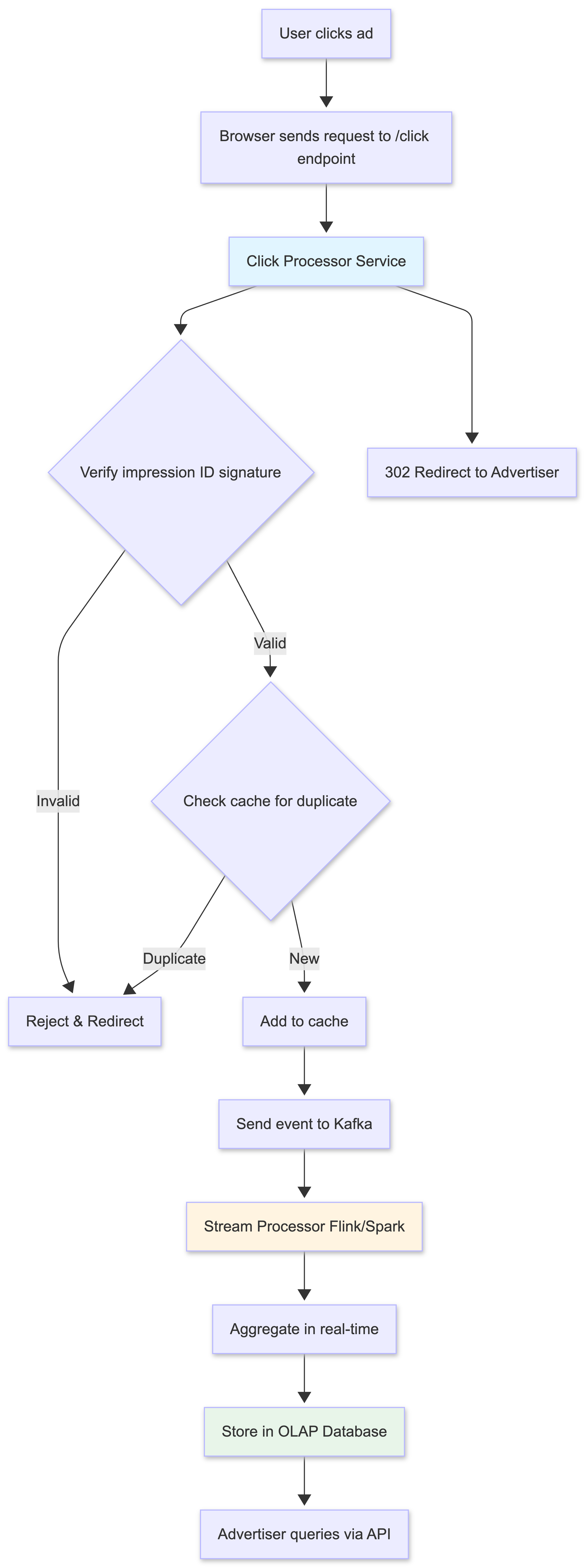
- User clicks on an ad on a website or app.
- The click is tracked - The browser sends a request to our
/clickendpoint with click data and impression ID. - Click Processor Service handles the request:
- Verifies the impression ID signature
- Checks for duplicates in cache
- Sends the click event to Kafka stream
- Responds with 302 redirect to advertiser’s website
- The user is redirected to the advertiser’s website.
- Stream Processor reads events from Kafka and aggregates them in real-time.
- Aggregated data is stored in the OLAP database.
- Advertisers query the system for aggregated click metrics via our APIs.
1. Users can click on ads and be redirected to the target
When a user clicks on an ad in their browser, we need to make sure that they’re redirected to the advertiser’s website. We assume there’s an existing Ad Placement Service (outside the scope of our design) which is responsible for placing ads on the website and associating them with the correct redirect URL.
When a user clicks on an ad which was placed by the Ad Placement Service, we will send a request to our /click endpoint, which will track the click and then redirect the user to the advertiser’s website.
Handle Redirect:
There are two ways we can handle this redirect:
Approach 1: Simple (Client-side redirect)
- Send over a redirect URL with each ad that’s placed on the website. When a user clicks on the ad, the browser will automatically redirect them to the target URL. We would then, in parallel, POST to our
/clickendpoint to track the click. - Challenge: Users could go to an advertiser’s website without us knowing about it, leading to discrepancies in click data.
Approach 2: Robust (Server-side redirect)
- Have the user click on the ad, which will then send a request to our server. Our server can then track the click and respond with a redirect to the advertiser’s website via a 302 (redirect) status code.
- Benefit: We can ensure that we track every click and provide a consistent experience. This approach also allows us to append additional tracking parameters to the URL.
- Challenge: The only downside is the added complexity, which could slow down the user experience. We need to make sure that our system can handle the additional load and respond quickly.
We recommend Approach 2 for better data accuracy.
2. Asynchronous Processing
If we were to implement a simple synchronous design, the Click Processor Service would directly call the Aggregation Service, which would then write to the database - all in a single request-response chain. However, this synchronous approach is not good because the capacity of producers and consumers is not always equal. Consider the following case; if there is a sudden increase in traffic and the number of events produced is far beyond what consumers can handle, consumers might get out-of-memory errors or experience an unexpected shutdown. If one component in the synchronous link is down, the whole system stops working.
A common solution is to adopt a message queue (Kafka) to decouple producers and consumers. This makes the whole process asynchronous and producers/consumers can be scaled independently.
The high-level design includes:
- Click Processor Service: Receives click events from users via HTTP requests, handles idempotency checking, and sends events to the message queue
- Message Queue (Kafka): Decouples producers and consumers
- Aggregation Service: Processes events and generates aggregated results
- Database Writer: Polls data from the message queue, transforms the data into the database format, and writes it to the database
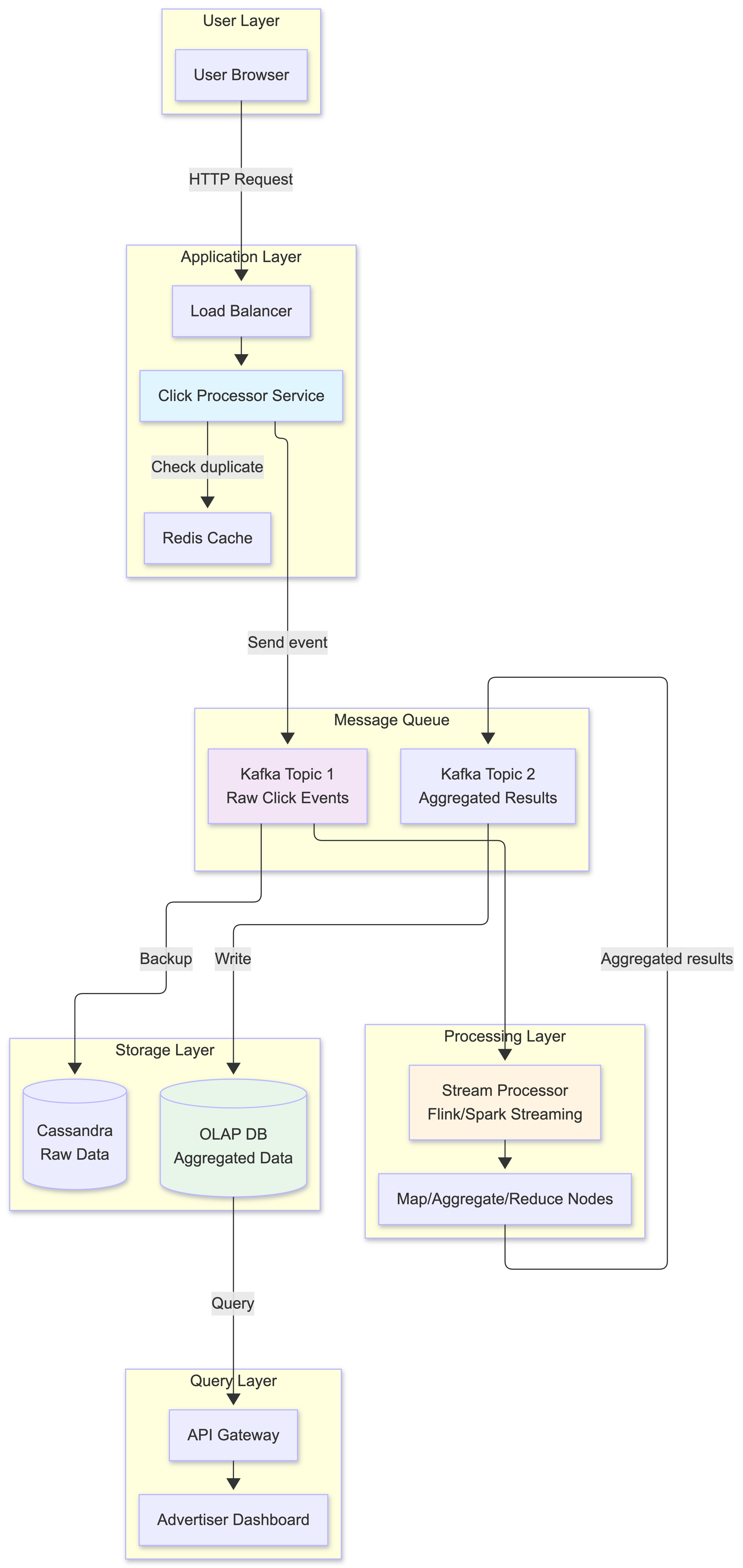
What is stored in the first message queue?
It contains ad click event data: ad_id, click_timestamp, user_id, ip, country, impression_id.
What is stored in the second message queue? The second message queue contains two types of data:
- Ad click counts aggregated at per-minute granularity:
ad_id,click_minute,count - Top N most clicked ads aggregated at per-minute granularity:
update_time_minute,most_clicked_ads
You might be wondering why we don’t write the aggregated results to the database directly. The short answer is that we need the second message queue like Kafka to achieve end-to-end exactly-once semantics (atomic commit).
How does the second message queue enable exactly-once semantics?
You might ask: “Why not use Kafka’s transactional producer directly with the database?” The key challenges are:
-
Database compatibility: Not all databases support distributed transactions with Kafka. Even if they do, cross-system transactions are complex and can impact performance.
-
Separation of concerns: The Aggregation Service focuses on stream processing logic, while the Database Writer handles database-specific optimizations (batching, retries, connection pooling).
The two-queue approach works as follows:
- Aggregation Service: Uses Kafka’s transactional producer to atomically:
- Commit the read offset from the first queue (input events)
- Write aggregated results to the second queue
If either operation fails, both are rolled back - no data loss or duplication at this stage.
- Database Writer: Reads from the second queue and writes to database. Since Kafka guarantees message delivery and we have idempotency keys (impression_id), the Database Writer can safely retry failed writes without creating duplicates.
This approach leverages Kafka’s strong consistency guarantees while keeping the database operations separate and optimizable. The second queue acts as a durable, transactional buffer between stream processing and database storage.
Aggregation Service
The MapReduce framework is a good option to aggregate ad click events. The directed acyclic graph (DAG) is a good model for it. The key to the DAG model is to break down the system into small computing units, like the Map/Aggregate/Reduce nodes.
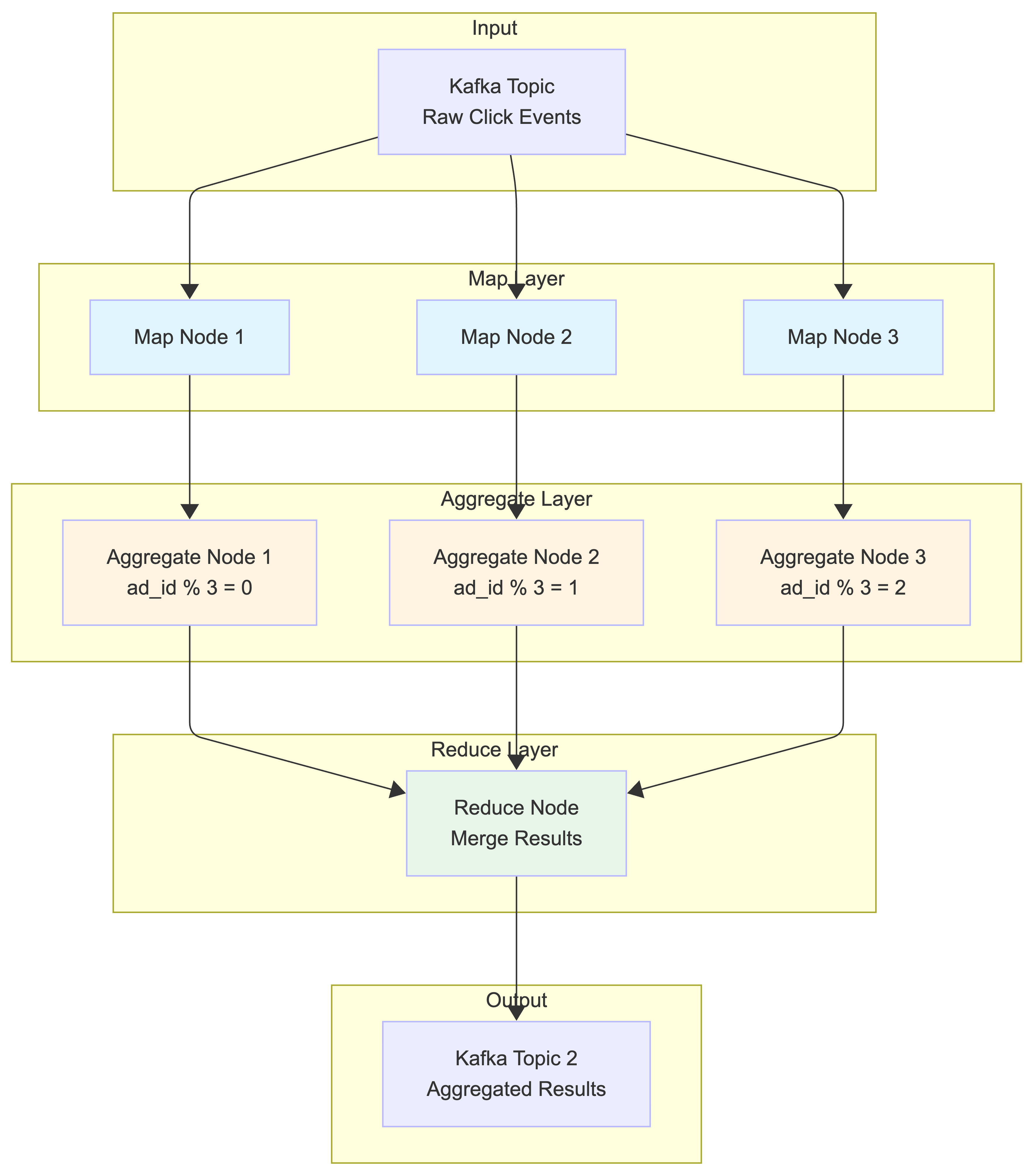
Map Node
A Map node reads data from a data source, and then filters and transforms the data. For example, a Map node sends ads with ad_id % 2 = 0 to Aggregation node 1, and the other ads go to Aggregation node 2.
You might be wondering why we need the Map node. An alternative option is to set up Kafka partitions and let the aggregate nodes subscribe to Kafka directly. This works, but there are several practical challenges:
-
Data cleaning and normalization: Raw click events might have inconsistent formats, missing fields, or invalid data that needs to be cleaned before aggregation. The Map node handles this preprocessing.
-
Lack of control over data production: In large organizations, multiple teams or services might produce click events to the same Kafka topic. For example:
- Web team produces events with partition key =
user_id(for user analytics) - Mobile team produces events with partition key =
session_id(for session tracking) - Ad serving team produces events with partition key =
campaign_id(for campaign optimization)
Even though all events contain
ad_id, they end up in different partitions based on different keys. This means events for the samead_id(e.g., “nike_001”) could be scattered across multiple partitions, making aggregation byad_idimpossible without reshuffling. - Web team produces events with partition key =
The Map node solves this by re-partitioning the data based on ad_id, ensuring that all events for the same ad go to the same Aggregate node, regardless of how the original data was partitioned.
Aggregate Node
An Aggregate node counts ad click events by ad_id in memory every minute.
Aggregation Window Logic:
Each Aggregate node uses tumbling windows based on event timestamps:
- Window boundaries: 00:00:00-00:00:59, 00:01:00-00:01:59, etc.
- Event assignment: Events are assigned to windows based on their
click_timestamp, not arrival time - Window processing: When system time reaches the end of a window + watermark (e.g., 00:01:15), the node:
- Finalizes aggregation for the previous window (00:00:00-00:00:59)
- Sends results to Reduce node
- Clears in-memory counters
- Starts fresh counters for the current window
Handling Late Events:
Example: Current system time is 00:01:10
- Event with timestamp 00:00:45 arrives → Added to previous window (still open due to 15s watermark)
- Event with timestamp 00:00:30 arrives at 00:01:20 → Dropped (window already closed)
- Event with timestamp 00:01:05 arrives → Added to current window
This ensures events are aggregated based on when they actually occurred, not when they arrived at our system.
How Aggregate Nodes work:
Each Aggregate node maintains an in-memory hash map that tracks click counts for each ad_id within its assigned partition. Let’s see an example:
Aggregate Node 1 (handles ad_id % 3 = 0):
Input events in 1 minute:
- ad_003: 150 clicks
- ad_006: 89 clicks
- ad_009: 234 clicks

In-memory aggregation:
{
  "ad_003": 150,
  "ad_006": 89,
  "ad_009": 234
}

Output to Reduce Node:
- Top 2 ads: [("ad_009", 234), ("ad_003", 150)]
- Total clicks: 473
Aggregate Node 2 (handles ad_id % 3 = 1):
Input events in 1 minute:
- ad_001: 312 clicks
- ad_004: 67 clicks
- ad_007: 198 clicks

Output to Reduce Node:
- Top 2 ads: [("ad_001", 312), ("ad_007", 198)]
- Total clicks: 577
Reduce Node
A Reduce node combines aggregated results from all Aggregate nodes to produce the final system-wide results.
Example: Finding Top 3 Most Clicked Ads
The Reduce node receives partial results from all Aggregate nodes:
Input from Aggregate Nodes:
- Node 1: [("ad_009", 234), ("ad_003", 150)]
- Node 2: [("ad_001", 312), ("ad_007", 198)]
- Node 3: [("ad_002", 445), ("ad_005", 123)]

Reduce Logic:
1. Merge all results: [("ad_002", 445), ("ad_001", 312), ("ad_009", 234), ("ad_007", 198), ("ad_003", 150), ("ad_005", 123)]
2. Sort by click count: [("ad_002", 445), ("ad_001", 312), ("ad_009", 234), ...]
3. Take top 3: [("ad_002", 445), ("ad_001", 312), ("ad_009", 234)]

Final Output:
{
  "timestamp": "2021-01-01T00:01:00Z",
  "top_ads": [
    {"ad_id": "ad_002", "clicks": 445},
    {"ad_id": "ad_001", "clicks": 312},
    {"ad_id": "ad_009", "clicks": 234}
  ]
}
Example: Aggregating Total Clicks by Filter
For filtered aggregations (e.g., US-only clicks), the process is similar:
Input from Aggregate Nodes (US filter):
- Node 1: {"ad_003": 89, "ad_006": 45}
- Node 2: {"ad_001": 156, "ad_004": 23}
- Node 3: {"ad_002": 234, "ad_005": 67}

Reduce Output:
{
  "timestamp": "2021-01-01T00:01:00Z",
  "filter_id": "US_ONLY",
  "aggregated_counts": [
    {"ad_id": "ad_002", "clicks": 234},
    {"ad_id": "ad_001", "clicks": 156},
    {"ad_id": "ad_003", "clicks": 89},
    ...
  ]
}
The DAG model represents the well-known MapReduce paradigm. It is designed to take big data and use parallel distributed computing to turn big data into little- or regular-sized data. Each stage processes data independently and in parallel, making the system highly scalable.
Step 3: Design Deep Dive
In this section, we will dive deep into the following:
- Streaming vs batching
- Time and aggregation window
- Delivery guarantees
- Scale the system
- Data monitoring and correctness
- Fault tolerance
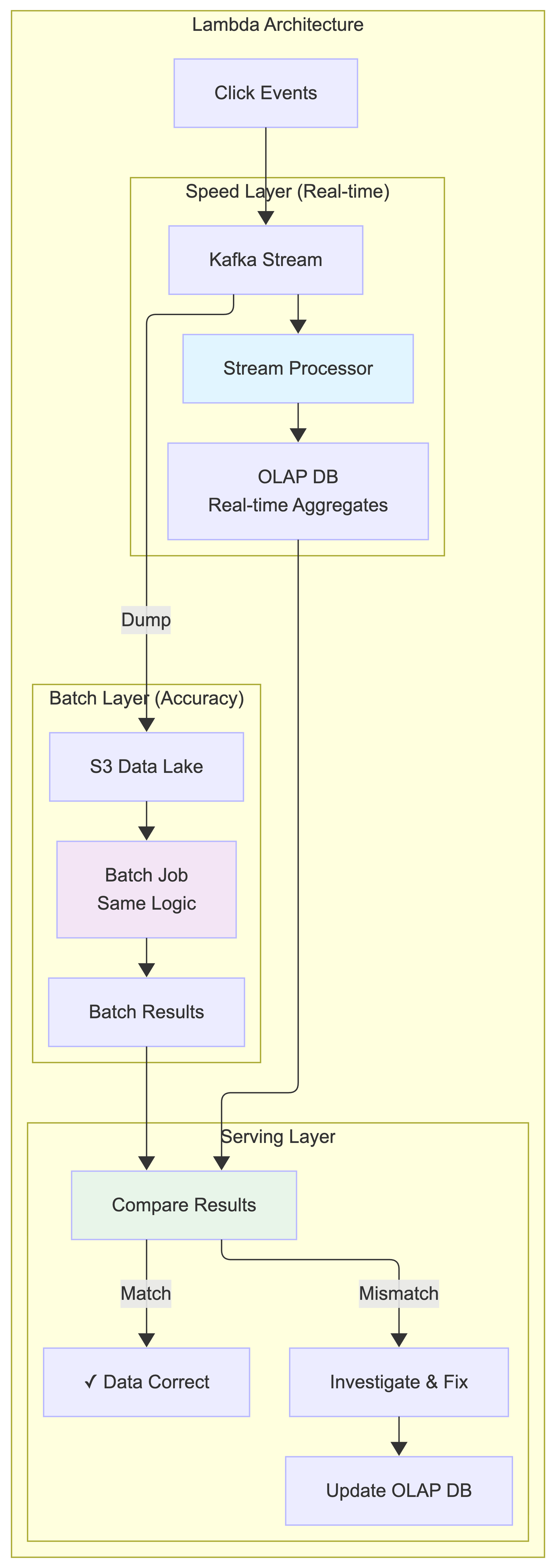
Streaming vs Batching
Our system uses stream processing as the primary approach to handle real-time ad click aggregation, with batch processing as a secondary mechanism for data reconciliation and historical replay.
Primary Path: Stream Processing
When a click comes in:
- The Click Processor Service writes the event to Kafka
- Stream processor reads events and aggregates them in real-time
- Aggregated results are written to the second Kafka topic
- Database Writer consumes from the second topic and writes to OLAP database
- Advertisers query the OLAP database for near real-time metrics
Secondary Path: Batch Processing (for reconciliation)
Simultaneously, we also:
- Dump raw click events from Kafka to S3 data lake
- Run daily batch jobs to re-aggregate the same data
- Compare batch results with stream processing results
- Identify and fix any discrepancies
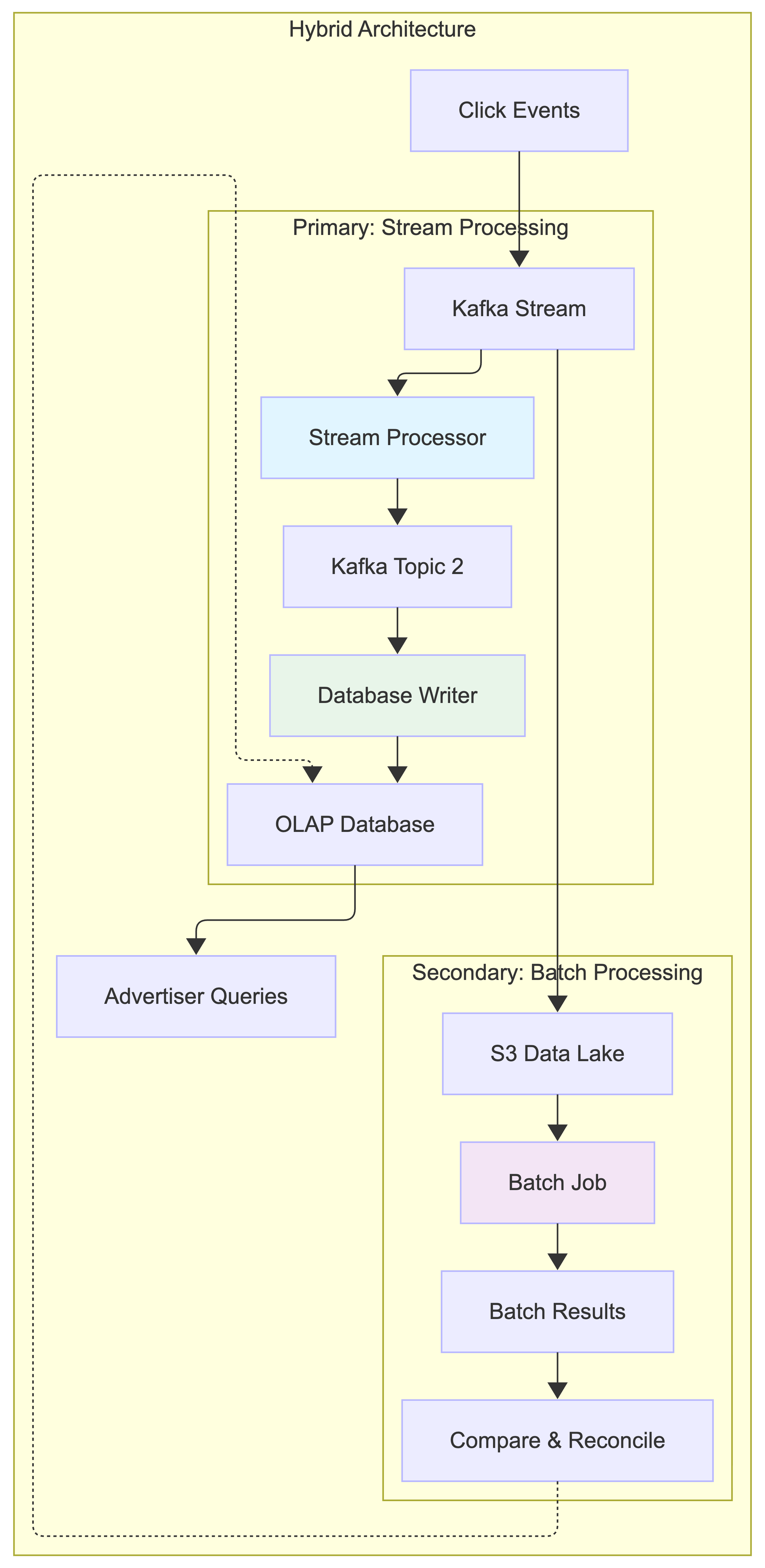
Architecture Classification:
This is essentially a Lambda Architecture with two processing paths:
- Speed layer: Stream processing for real-time results
- Batch layer: Batch processing for accurate historical processing
- Serving layer: OLAP database that serves both results
However, we minimize the complexity by using the same aggregation logic in both stream and batch processing, reducing code duplication.
Historical Data Replay:
When we need to recalculate historical data (e.g., after fixing a bug):
Option 1: Shared Logic Approach
- Extract the aggregation logic into a shared library/module (e.g.,
AdClickAggregator) - Both stream processor and batch job use the same
AdClickAggregator.aggregate()function - For replay: Batch job reads raw data from S3 → calls
AdClickAggregator.aggregate()→ writes to OLAP DB - This ensures identical aggregation logic but different data sources (Kafka vs S3)
Option 2: Stream Replay Approach
- Write historical raw data from S3 back to a temporary Kafka topic
- Stream processor reads from this temporary topic (same as normal processing)
- Results go through the same pipeline: Stream processor → Kafka → Database Writer → OLAP DB
- Delete temporary topic after replay completes
Shared Logic Approach: Extract aggregation logic into a shared library (e.g., AdClickAggregator). Both stream processor and batch jobs use the same aggregate() function, ensuring consistent logic while using different data sources (Kafka vs S3).
Time: Event Time vs Processing Time
We need a timestamp to perform aggregation. The timestamp can be generated in two different places:
- Event time: when an ad click happens.
- Processing time: refers to the system time of the aggregation server that processes the click event.
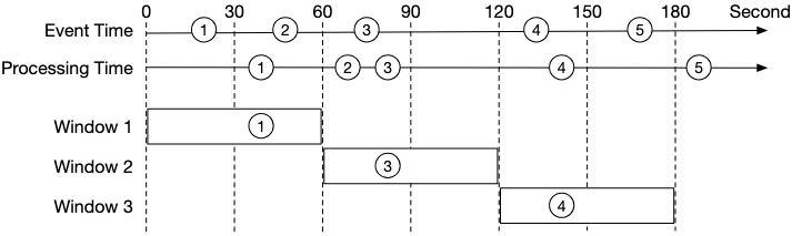
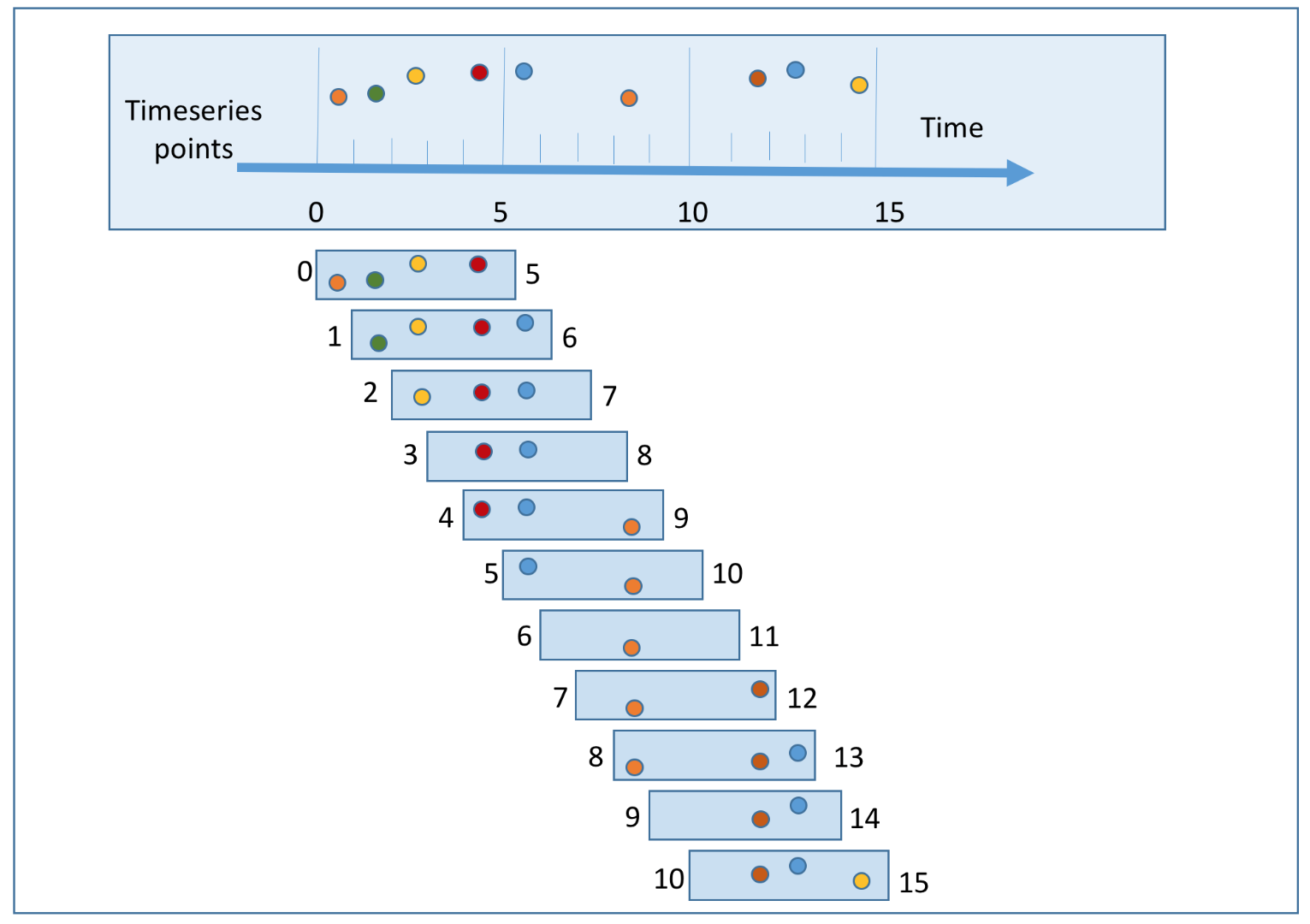
Due to network delays and asynchronous environments (data go through a message queue), the gap between event time and processing time can be large. As shown in the diagram below, events can arrive significantly later than when they actually occurred. For example, Event 2 happens at t=45s but arrives at t=70s (25 seconds delay), while Event 3 happens at t=75s but arrives much later at t=80s (5 seconds delay).
| Pros | Cons | |
|---|---|---|
| Event time | Aggregation results are more accurate because the client knows exactly when an ad is clicked | It depends on the timestamp generated on the client-side. Clients might have the wrong time, or the timestamp might be generated by malicious users |
| Processing time | Server timestamp is more reliable | The timestamp is not accurate if an event reaches the system at a much later time |
Since data accuracy is very important, we recommend using event time for aggregation. How do we properly process delayed events in this case? A technique called “watermark” is commonly utilized to handle slightly delayed events.
The Challenge: Missing Events in Aggregation Windows
When using event time for aggregation, we face a fundamental challenge: events can arrive out of order. Consider this scenario where we’re aggregating clicks in 30-second windows:
Example Timeline (in seconds):
- Window 1: t=0s - t=59s
- Window 2: t=60s - t=119s
- Window 3: t=120s - t=179s
Events arriving at the aggregation service (as shown in the diagram):
- Event 1:
click_timestamp=t=20s,arrival_time=t=40s→ ✅ Belongs to Window 1 (0-59s), arrives on time (20s delay) - Event 2:
click_timestamp=t=50s,arrival_time=t=70s→ ❌ Belongs to Window 1 (0-59s), arrives late (20s delay, Window 1 has closed) - Event 3:
click_timestamp=t=75s,arrival_time=t=80s→ ✅ Belongs to Window 2 (60-119s), arrives on time (5s delay) - Event 4:
click_timestamp=t=135s,arrival_time=t=140s→ ✅ Belongs to Window 3 (120-179s), arrives on time (5s delay) - Event 5:
click_timestamp=t=165s,arrival_time=t=190s→ ❌ Belongs to Window 3 (120-179s), arrives very late (25s delay, Window 3 has already closed)

The Problem (as illustrated in the diagram):
- If we close Window 1 at exactly t=60s (without watermark), we miss Event 2 (which happened at t=50s but arrives at t=70s)
- If we close Window 3 at exactly t=180s (without watermark), we miss Event 5 (which happened at t=165s but arrives at t=190s)
- This leads to undercounting and inaccurate aggregation results
Why do events arrive late?
- Network delays: Packets can be delayed or take different routes
- Client-side buffering: Mobile apps might batch events and send them later
- Message queue processing: Kafka partitions might have different processing speeds
- System failures: Temporary outages can cause event backlogs
- Geographic distribution: Events from different regions have varying latencies
Watermark Technique: The Solution
One way to mitigate this problem is to use “watermark” (the extended rectangles in the diagram below), which is regarded as an extension of an aggregation window. This improves the accuracy of the aggregation result. As shown in the diagram, by extending an extra 15-second (adjustable) aggregation window:
- Window 1 (closes at t=74s with 15s watermark): Can catch Event 1 (arrives at t=40s) and Event 2 (arrives at t=70s, both belong to Window 1)
- Window 2 (closes at t=134s with 15s watermark): Can catch Event 3 (arrives at t=80s, belongs to Window 2)
- Window 3 (closes at t=194s with 15s watermark): Can catch Event 4 (arrives at t=140s) and Event 5 (arrives at t=190s, both belong to Window 3)
With a 15-second watermark, all events in our example are successfully caught, demonstrating how watermarks help handle late-arriving events.
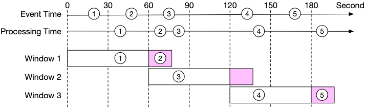
How Watermarks Work:
A watermark is essentially a grace period that extends each aggregation window. Instead of immediately closing a window when its time boundary is reached, we wait for an additional period (the watermark) to catch late-arriving events.
Detailed Example with 15-second Watermark (matching the diagram):
Window 1: t=0s - t=59s (+ 15s watermark = closes at t=74s)
Window 2: t=60s - t=119s (+ 15s watermark = closes at t=134s)
Window 3: t=120s - t=179s (+ 15s watermark = closes at t=194s)
Event Processing Timeline (matching the diagram):
| System Time | Event | Event Timestamp | Arrival Time | Window Assignment | Status |
|---|---|---|---|---|---|
| t=40s | Event 1 | t=20s | t=40s | Window 1 (0-59s) | ✅ On time (20s delay, arrives before window closes at t=74s) |
| t=70s | Event 2 | t=50s | t=70s | Window 1 (0-59s) | ✅ Late but within watermark (20s delay, arrives at t=70s before window closes at t=74s - CAUGHT) |
| t=74s | - | - | - | Window 1 closes | Final count: 2 events |
| t=80s | Event 3 | t=75s | t=80s | Window 2 (60-119s) | ✅ On time (5s delay, arrives before window closes at t=134s) |
| t=134s | - | - | - | Window 2 closes | Final count: 1 event |
| t=140s | Event 4 | t=135s | t=140s | Window 3 (120-179s) | ✅ On time (5s delay, arrives before window closes at t=194s) |
| t=190s | Event 5 | t=165s | t=190s | Window 3 (120-179s) | ✅ Late but within watermark (25s delay, arrives at t=190s before window closes at t=194s - CAUGHT) |
| t=194s | - | - | - | Window 3 closes | Final count: 2 events |
Note: With a 15-second watermark, all events are successfully caught:
- Window 1: Event 1 and Event 2 are both included (Event 2 arrives late but within watermark)
- Window 2: Event 3 is included (arrives on time)
- Window 3: Event 4 and Event 5 are both included (Event 5 arrives late but within watermark)
Watermark Implementation Concept:
A watermark extends each window’s closing time. Events are accepted if they belong to the window’s time range AND arrive before the watermark expires. For example, Window 1 (0-59s) with 15s watermark closes at t=74s, catching events that arrive up to 15 seconds late.
Watermark Configuration: Balancing Accuracy vs Latency
The value set for the watermark depends on the business requirement. This creates a fundamental trade-off:
Long Watermark (e.g., 5 minutes):
- ✅ Higher accuracy: Catches most late-arriving events
- ✅ Better completeness: Reduces data loss from network delays
- ❌ Higher latency: Advertisers wait longer for aggregated results
- ❌ Increased memory usage: More windows kept open simultaneously
- ❌ Delayed billing: Revenue recognition is postponed
Short Watermark (e.g., 15 seconds):
- ✅ Lower latency: Faster results for real-time dashboards
- ✅ Reduced memory usage: Windows close quickly
- ✅ Faster billing cycles: Quicker revenue recognition
- ❌ Lower accuracy: Some late events are still missed
- ❌ Potential revenue loss: Undercounting can affect billing
Choosing the Right Watermark Duration:
The optimal watermark duration should be based on:
- Historical latency analysis: Analyze your system’s 95th or 99th percentile event arrival delays
- Business requirements: How much latency can advertisers tolerate?
- Financial impact: What’s the cost of missing 1% vs 0.1% of events?
- System resources: How much memory can you allocate to keep windows open?
Example Analysis:
Historical Event Arrival Delays (last 30 days):
- 50th percentile: 2 seconds
- 90th percentile: 8 seconds
- 95th percentile: 15 seconds
- 99th percentile: 45 seconds
- 99.9th percentile: 3 minutes

Recommendation: 15-second watermark captures 95% of late events
with acceptable latency for real-time dashboards.
Advanced Watermark Strategies
1. Dynamic Watermarks: Adjust based on current system conditions (increase during high load, decrease during low load)
2. Per-Source Watermarks: Different durations for different sources (mobile: 30s, web: 10s, server: 5s)
3. Tiered Processing: Process events in multiple passes with different watermarks to balance speed and accuracy:
Instead of using a single watermark, process the same data multiple times with increasingly longer watermarks. This gives advertisers quick preliminary results while ensuring high accuracy for final billing.
Example:
- Pass 1 (5s watermark): Quick results for real-time dashboards (low latency, lower accuracy)
- Pass 2 (60s watermark): More accurate results for campaign optimization (higher latency, better accuracy)
- Pass 3 (End of day batch): Final reconciliation from S3 data lake for billing (highest accuracy)
Each pass uses the same Kafka stream but with different consumer groups and watermark durations, allowing progressive refinement of results over time.
Handling Events with Extreme Delays
Notice that the watermark technique does not handle events that have long delays (hours or days). We can argue that it is not worth the return on investment (ROI) to have a complicated design for low probability events. We can always correct the tiny bit of inaccuracy with end-of-day reconciliation (see Reconciliation section).
Why not handle extremely late events?
- Diminishing returns: Events arriving hours late represent <0.01% of total volume
- System complexity: Supporting arbitrary delays requires complex state management
- Memory costs: Keeping windows open for hours consumes significant resources
- Business impact: The financial impact of missing these rare events is minimal
Alternative approaches for extreme delays:
- Batch reconciliation: Run daily batch jobs to catch and correct missed events
- Separate late-event pipeline: Process extremely late events in a different system
- Statistical correction: Apply correction factors based on historical late-event patterns
One trade-off to consider is that using watermark improves data accuracy but increases overall latency, due to extended wait time.
Real-world Example:
Consider a major advertising platform processing 1 billion clicks per day:
- Without watermarks: 99.2% accuracy, 1-second latency
- With 15s watermarks: 99.8% accuracy, 16-second latency
- With 60s watermarks: 99.95% accuracy, 61-second latency
The business decision depends on whether the 0.6% accuracy improvement (from 99.2% to 99.8%) justifies the 15x latency increase (1s to 16s) for real-time advertising decisions.
Aggregation Window
According to “Designing data-intensive applications” by Martin Kleppmann, there are four types of window functions: tumbling (also called fixed) window, hopping window, sliding window, and session window. We will discuss the tumbling window and sliding window as they are most relevant to our system.
- Tumbling window: Time is partitioned into same-length, non-overlapping chunks. The tumbling window is a good fit for aggregating ad click events every minute (use case 1).
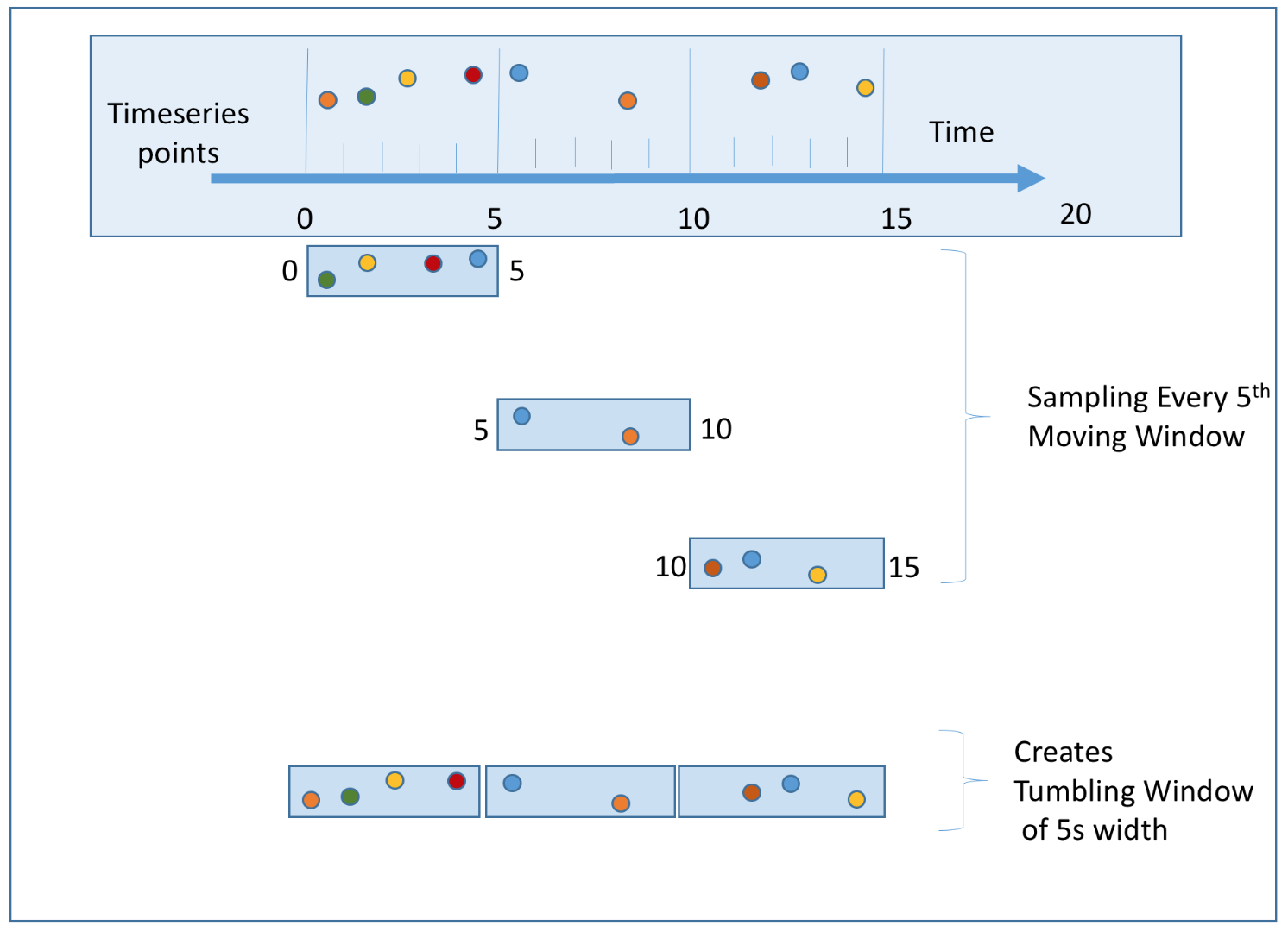
- Sliding window: Events are grouped within a window that slides across the data stream, according to a specified interval. A sliding window can be an overlapping one. This is a good strategy to satisfy our second use case; to get the top N most clicked ads during the last M minutes.
Delivery Guarantees: Exactly-Once Semantics
Since the aggregation result is utilized for billing, data accuracy and completeness are very important. The system needs to be able to answer questions such as:
- How to avoid processing duplicate events?
- How to ensure all events are processed?
Message queues such as Kafka usually provide three delivery semantics: at-most once, at-least once, and exactly once.
Which delivery method should we choose?
In most circumstances, at-least once processing is good enough if a small percentage of duplicates are acceptable. However, this is not the case for our system. Differences of a few percent in data points could result in discrepancies of millions of dollars. Therefore, we recommend exactly-once delivery for the system.
Data Deduplication
One of the most common data quality issues is duplicated data. There are two types of duplication we need to handle:
Type 1: Multiple Events Generated (Client-side Duplication)
This happens when the same user action generates multiple click events:
- User double-clicks: User accidentally clicks the same ad multiple times in quick succession
- Network retries: Browser automatically retries failed requests, sending the same click multiple times
- Mobile app issues: App sends the same click event multiple times due to connectivity issues
- Malicious behavior: Fraudulent clicks sent with malicious intent (handled by fraud detection)
Type 2: Same Event Processed Multiple Times (System-side Duplication)
This happens when a single event gets processed multiple times by our system:
- Stream processor restarts: When processor crashes and restarts, it replays events from last checkpoint
- Multiple processing passes: Tiered processing with different watermarks can process the same event multiple times. A duplicate event may arrive too late for the first tier’s window, but the second tier, with a longer watermark, can still include it.
- Distributed processing: Same event processed by multiple nodes due to partitioning issues
- Network failures: Upstream service resends events when it doesn’t receive acknowledgment
Why Dedup Before Stream Processing?
We need to dedup before we put the click in the stream (at Click Processor Service level) to handle both types of duplication:
Type 1: Prevents multiple events from same user action from entering the stream Type 2: Ensures each unique event only enters the stream once, so even if stream processor replays events, there are no duplicates to replay. This is handled by our exactly-once semantics using the 2 message queues architecture mentioned above:
- The first queue to aggregation service uses Kafka’s transactional producer
- The second queue to database writer ensures atomic commits
- This prevents the same event from being processed multiple times even during system failures or restarts
By combining early deduplication (for Type 1) with exactly-once semantics (for Type 2), we ensure each unique user click is counted exactly once.
Implementation Flow:
- Ad Placement Service generates a unique impression ID for each ad instance shown to the user.
- The impression ID is signed with a secret key and sent to the browser along with the ad.
- When the user clicks on the ad, the browser sends a request to our
/clickendpoint with the impression ID along with the click data. - The Click Processor Service:
- Verifies the signature of the impression ID to ensure it’s valid (prevents fake clicks with falsified impression IDs)
- Checks if the impression ID exists in a distributed cache (like Redis Cluster or Memcached). If it does, then it’s a duplicate, and we ignore it and still redirect the user.
- If it doesn’t exist, we put the click event in the Kafka stream and add the impression ID to the cache with a TTL (e.g., 24 hours)
- Responds with a 302 redirect to the advertiser’s website
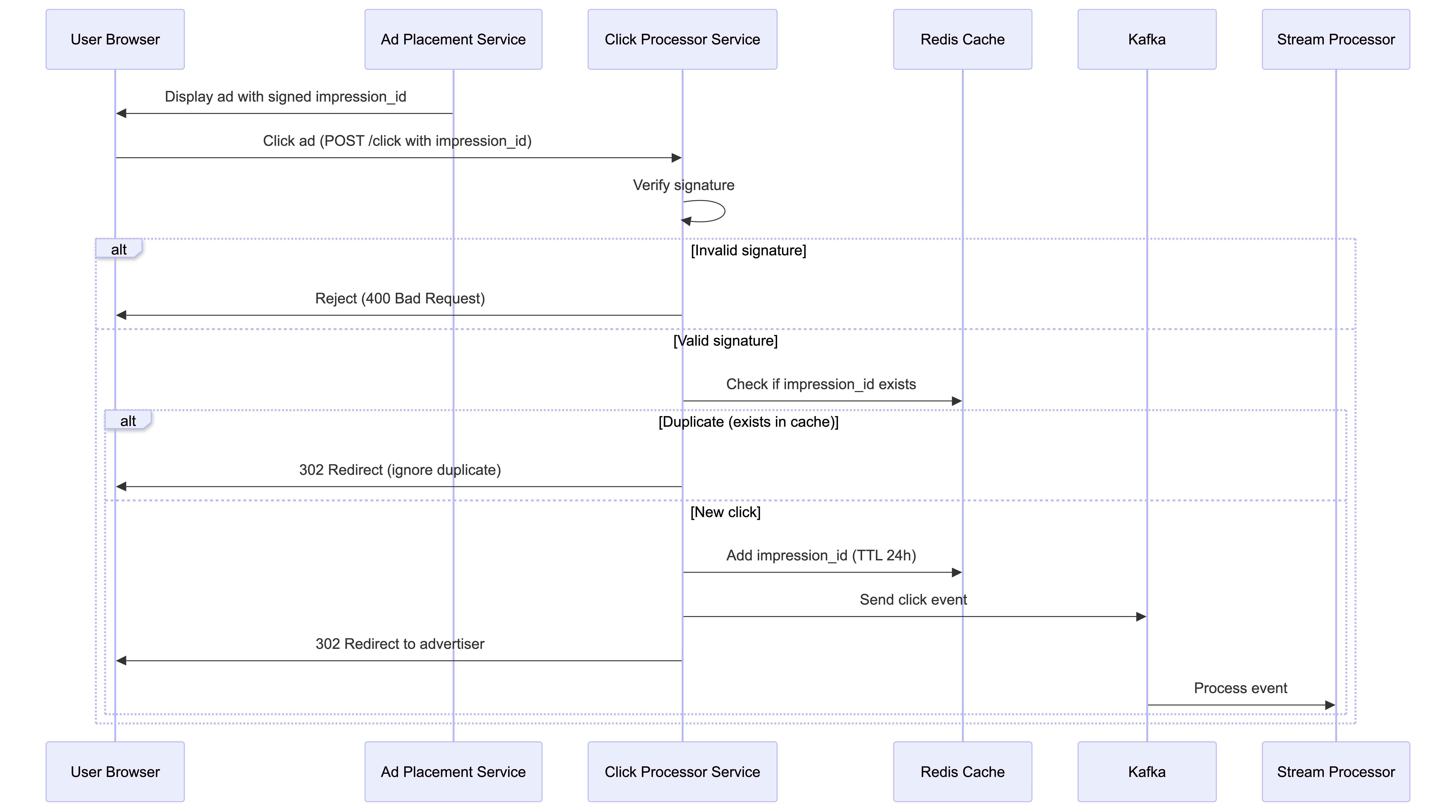
Why sign the impression ID? A malicious user could send a bunch of fake clicks with falsified impression IDs. Because they’d all be unique, our current solution would count them all. By signing the impression ID with a secret key, we can verify the signature to ensure the impression ID is valid before checking the cache.
Cache Considerations: The cache data should be relatively small. With 100 million clicks per day, if these were all unique impressions, then that’s only 100 million * 16 bytes (128 bits) = 1.6 GB. Tiny. We can easily scale this using a distributed cache like Redis Cluster or Memcached. In the event the cache goes down, we would handle this by having a replica of the cache that could take over and by enabling cache persistence so the cache data is not lost.
Alternative Approach: Bloom Filters
For extremely high-scale scenarios where memory efficiency is critical, we can use Bloom Filters as an alternative or complementary approach:
How Bloom Filters Work:
- Probabilistic data structure that can tell if an impression ID “definitely not seen” or “possibly seen”
- Memory usage: ~10 bits per element (vs 128 bits for storing full impression ID)
- Trade-off: Small false positive rate (might reject ~0.1% of legitimate clicks) but no false negatives
- Example: 100M impressions need only ~120MB instead of 1.6GB
Implementation Strategy:
- Two-tier approach: Use Bloom Filter as a pre-filter before checking Redis
- Process: Check Bloom Filter first → if “definitely not seen”, accept click → if “possibly seen”, check Redis for exact verification
- Benefit: Reduces Redis load by 99%+ while maintaining exact deduplication accuracy
When to Use:
- Redis Cache: When exact accuracy is required (recommended for billing)
- Bloom Filter: When memory is extremely constrained and small error rate is acceptable
- Hybrid: Bloom Filter + Redis for memory optimization with exact accuracy
Scale the System
From the back-of-the-envelope estimation, we know the business grows 30% per year, which doubles traffic every 3 years. How do we handle this growth?
Our system consists of four independent components: click processor service, message queue, aggregation service, and database. Since these components are decoupled, we can scale each one independently.
Scale the Click Processor Service
Click Processor Service: We can easily scale this service horizontally by adding more instances. Most modern cloud providers like AWS, Azure, and GCP provide managed services that automatically scale services based on CPU or memory usage. We’ll need a load balancer in front of the service to distribute the load across instances.
Scale the Message Queue
Producers: The Click Processor Service instances act as producers. We don’t limit the number of producer instances, so the scalability of producers can be easily achieved.
Consumers: Inside a consumer group, the rebalancing mechanism helps to scale the consumers by adding or removing nodes. By adding more consumers, each consumer only processes events from one partition.
When there are hundreds of Kafka consumers in the system, consumer rebalance can be quite slow and could take a few minutes or even more. Therefore, if more consumers need to be added, try to do it during off-peak hours to minimize the impact.
Brokers:
- Hashing key: Using
ad_idas hashing key for Kafka partition to store events from the samead_idin the same Kafka partition. In this case, an aggregation service can subscribe to all events of the samead_idfrom one single partition. Sharding byad_idis a natural choice, this way, the stream processor can read from multiple shards in parallel since they will be independent of each other (all events for a givenad_idwill be in the same shard). - The number of partitions: If the number of partitions changes, events of the same
ad_idmight be mapped to a different partition. Therefore, it’s recommended to pre-allocate enough partitions in advance, to avoid dynamically increasing the number of partitions in production. - Topic physical sharding: One single topic is usually not enough. We can split the data by geography (topic_north_america, topic_europe, topic_asia, etc.,) or by business type (topic_web_ads, topic_mobile_ads, etc).
- Stream capacity: Both Kafka and Kinesis are distributed and can handle a large number of events per second but need to be properly configured. Kinesis, for example, has a limit of 1MB/s or 1000 records/s per shard, so we’ll need to add some sharding.
Scale the Aggregation Service
The stream processor can also be scaled horizontally by adding more tasks or jobs. We’ll have separate jobs reading from each shard doing the aggregation for the ad_ids in that shard.
Aggregation service is horizontally scalable by adding or removing nodes. There are two options to increase the throughput:
- Option 1: Allocate events with different
ad_idsto different threads (multi-threading). - Option 2: Deploy aggregation service nodes on resource providers like Apache Hadoop YARN (multi-processing).
Option 1 is easier to implement and doesn’t depend on resource providers. In reality, however, option 2 is more widely used because we can scale the system by adding more computing resources.
Scale the Database
Raw Data Storage (Cassandra): Cassandra natively supports horizontal scaling, in a way similar to consistent hashing. Data is evenly distributed to every node with a proper replication factor. Each node saves its own part of the ring based on hashed value and also saves copies from other virtual nodes. If we add a new node to the cluster, it automatically rebalances the virtual nodes among all nodes. No manual resharding is required.
Aggregated Data Storage (OLAP Database): The OLAP database can be scaled horizontally by adding more nodes. While we could shard by ad_id, we may also consider sharding by advertiser_id instead. In doing so, all the data for a given advertiser will be on the same node, making queries for that advertiser’s ads faster. This is in anticipation of advertisers querying for all of their active ads in a single view. Of course, it’s important to monitor the database and query performance to ensure that it’s meeting the SLAs and adapting the sharding strategy as needed.
Query Latency Optimization: Pre-Aggregating Data
As mentioned in our non-functional requirements, advertisers need sub-second response time for querying aggregated data. Our real-time stream processing architecture already addresses this for recent time windows (minutes to hours) by pre-aggregating data at 1-minute granularity and storing it in the OLAP database. However, queries over larger time windows can still be slow.
The Problem: Large Time Window Queries
When advertisers query metrics over days, weeks, or months, the OLAP database needs to scan and aggregate millions of minute-level records. For example:
- Querying 1 day of data: 1,440 minute-level records per ad
- Querying 1 week of data: 10,080 minute-level records per ad
- Querying 1 month of data: ~43,200 minute-level records per ad
With 2 million active ads, aggregating a month of data across all ads requires processing billions of records, which can take several seconds or even minutes—far exceeding our sub-second SLA.
The Solution: Multi-Level Pre-Aggregation
We can pre-aggregate data at multiple granularity levels in the OLAP database, similar to a materialized view or caching strategy. This creates a hierarchy of aggregated tables:
| Granularity | Table Name | Aggregation Window | Use Case |
|---|---|---|---|
| Minute-level | ad_clicks_minute |
1 minute | Real-time dashboards, recent queries |
| Hourly | ad_clicks_hour |
1 hour | Daily reports, trend analysis |
| Daily | ad_clicks_daily |
1 day | Weekly/monthly reports, historical analysis |
| Weekly | ad_clicks_weekly |
1 week | Long-term trend analysis, quarterly reports |
Implementation:
- Real-time aggregation (existing): Stream processor writes minute-level aggregates to
ad_clicks_minutetable - Hourly rollup: A scheduled job runs every hour to aggregate the last 60 minutes from
ad_clicks_minuteintoad_clicks_hour - Daily rollup: A nightly cron job aggregates 24 hours from
ad_clicks_hourintoad_clicks_daily - Weekly rollup: A weekly job aggregates 7 days from
ad_clicks_dailyintoad_clicks_weekly
Query Strategy:
When an advertiser queries data, the system intelligently selects the appropriate table based on the time range:
Example: Query clicks for last 30 days
- Query ad_clicks_daily table (30 rows) instead of ad_clicks_minute (43,200 rows)
- Response time: <100ms (vs 5+ seconds for minute-level aggregation)
For drill-down scenarios, the system can query multiple tables:
- High-level view: Query
ad_clicks_dailyfor monthly trends - Detailed view: Query
ad_clicks_minutefor specific hours when needed
Trade-offs:
| Aspect | Impact |
|---|---|
| Query Performance | ✅ Dramatically faster for large time windows (10-100x improvement) |
| Storage Cost | ❌ Increases storage by ~15-20% (multiple aggregation levels) |
| Data Freshness | ⚠️ Hourly/daily aggregates have slight delay (acceptable for historical queries) |
| Complexity | ⚠️ Requires additional ETL jobs and query routing logic |
Pre-aggregation is a common technique in OLAP systems, trading storage space for query performance. Given that storage is relatively cheap compared to query latency’s impact on user experience, this is a worthwhile optimization for our system.
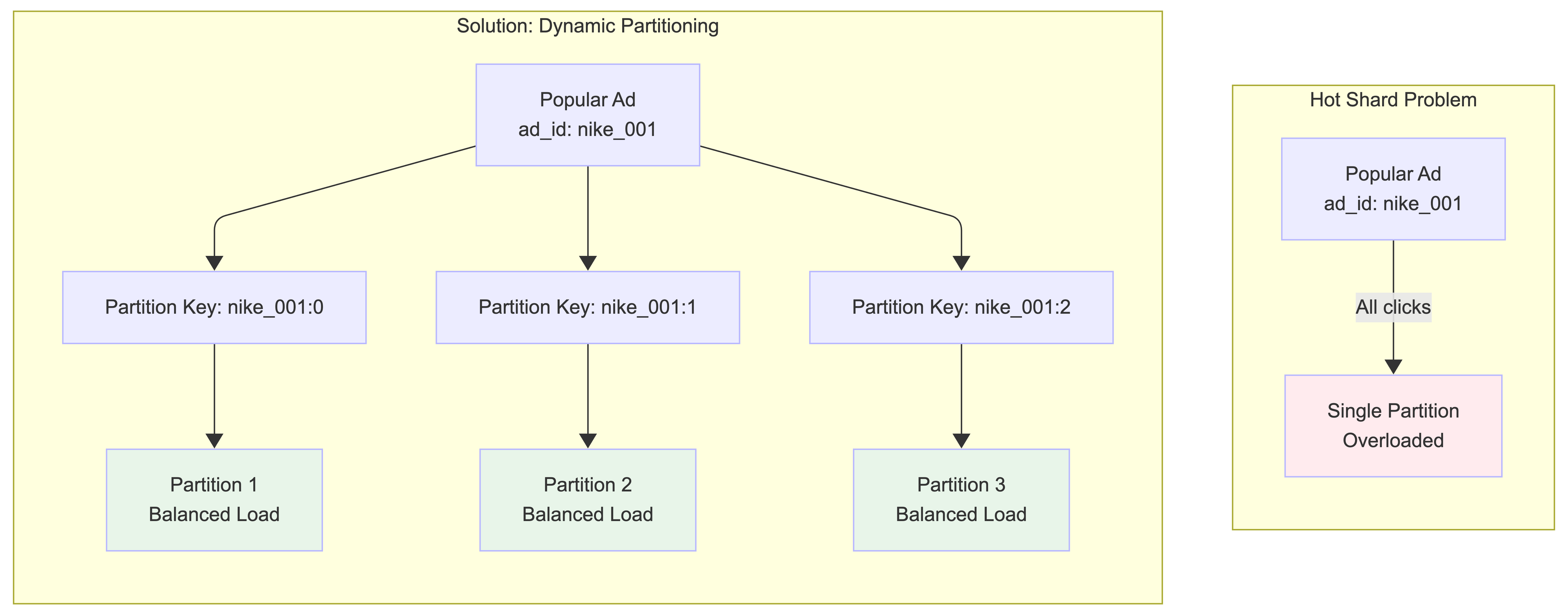
Hotspot Issue
A shard or service that receives much more data than the others is called a hotspot. This occurs because major companies have advertising budgets in the millions of dollars and their ads are clicked more often. Since events are partitioned by ad_id, hotspots can occur at two levels:
1. Hot Shards in Kafka Partitions:
When a popular ad (e.g., Nike’s new ad with Lebron James) gets many clicks, all events for that ad_id go to the same Kafka partition, overwhelming that partition.
Solution - Dynamic Partitioning:
Update the partition key by appending a random number to the ad_id for popular ads. The partition key becomes ad_id:0-N where N is the number of additional partitions for that ad_id. This distributes clicks for the same ad across multiple partitions.
2. Hot Nodes in Aggregation Service: Some aggregation service nodes might receive many more ad click events than others, potentially causing server overload.
Solution - Dynamic Resource Allocation: When an aggregation node is overloaded, it can request additional resources through the resource manager. The resource manager allocates more aggregation nodes, and the original node splits events into multiple groups for parallel processing. More sophisticated approaches include Global-Local Aggregation or Split Distinct Aggregation.
Fault Tolerance
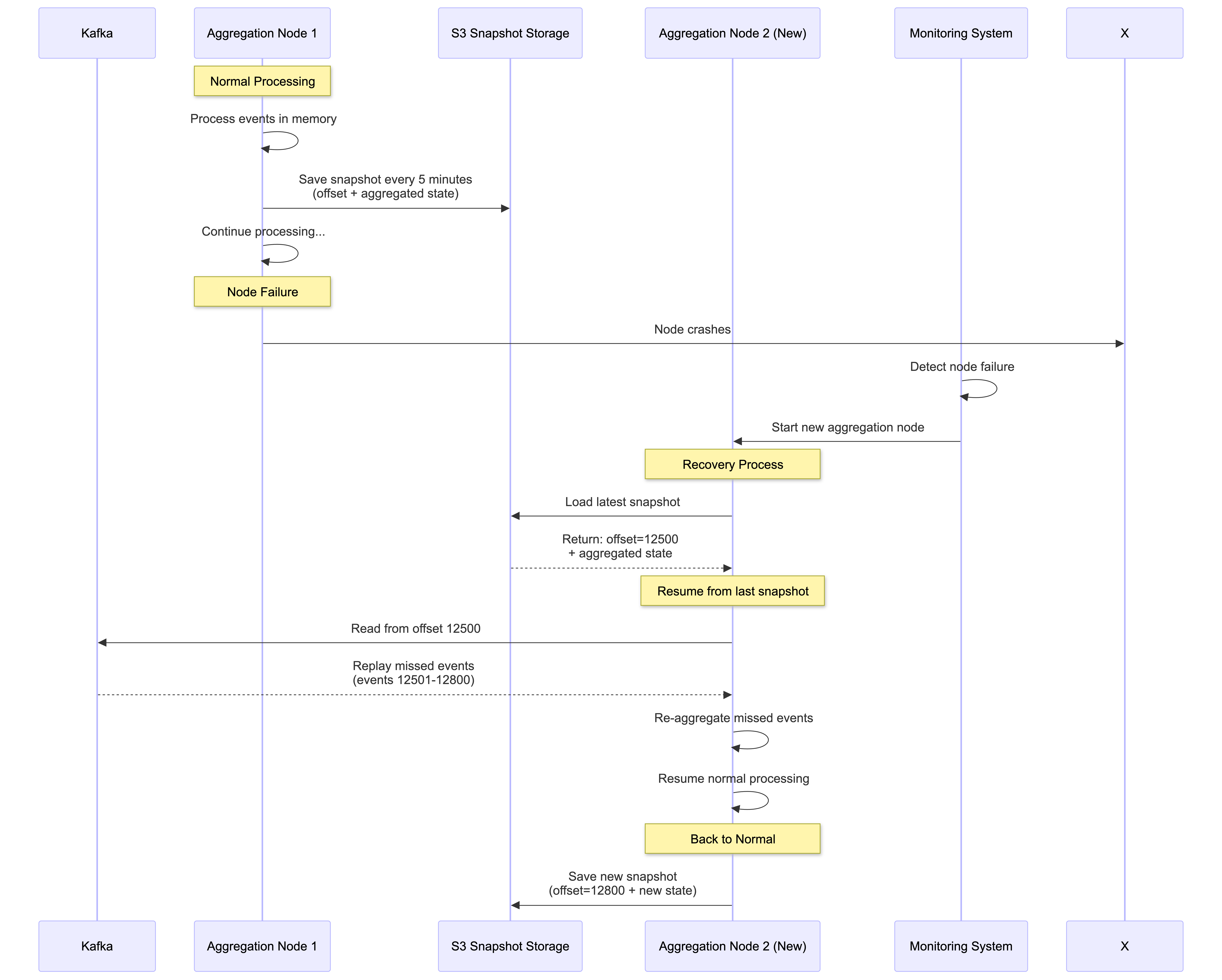
Let’s discuss the fault tolerance of the aggregation service. Since aggregation happens in memory, when an aggregation node goes down, the aggregated result is lost as well. We can rebuild the count by replaying events from upstream Kafka brokers.
Replaying data from the beginning of Kafka is slow. A good practice is to save the “system status” like upstream offset to a snapshot and recover from the last saved status. In our design, the “system status” is more than just the upstream offset because we need to store data like top N most clicked ads in the past M minutes.
With a snapshot, the failover process of the aggregation service is quite simple. If one aggregation service node fails, we bring up a new node and recover data from the latest snapshot. If there are new events that arrive after the last snapshot was taken, the new aggregation node will pull those data from the Kafka broker for replay.
Snapshot Contents:
- Kafka offset: Last processed event position (e.g., offset 12500)
- In-memory aggregation state: Current click counts per ad_id for active 30-second windows
- Window state: Top N most clicked ads in current time windows (e.g., top 10 ads in last 5 minutes)
- Watermark state: Current 5-second watermark positions for each active window
- Impression ID cache: Recent impression IDs for deduplication (with TTL)
- Timestamp: When the snapshot was taken
Recovery Timeline Example:
10:00:00 - Snapshot saved (offset: 12500, processing window 10:00:00-10:00:29)
10:00:15 - Node crashes (had processed 300 more events, watermark still open)
10:00:15 - Monitoring detects failure, starts new node
10:00:30 - New node loads snapshot, resumes from offset 12500
10:00:30 - Replays 300 missed events + processes late arrivals within 5s watermark
10:00:35 - Window 10:00:00-10:00:29 closes (watermark expired), fully recovered
Stream Retention Policy: We use Kafka to store click data with built-in fault tolerance. Kafka replicates data across multiple nodes and data centers, ensuring no data loss even if nodes fail. We configure a 7-day retention period, so if our stream processor goes down, it can recover and replay lost events from Kafka.
This retention policy works well with our 30-second aggregation windows and 5-second watermarks - even if a processor is down for hours, it can still recover all necessary events for accurate aggregation.
Checkpointing: Our stream processors use checkpointing to periodically save state to S3. However, given our small 30-second windows, if a processor fails, we lose at most 30 seconds of aggregated data. With Kafka persistence enabled, we can simply replay the lost click events and re-aggregate them quickly.
The combination of snapshots (for in-memory state) + checkpointing (for stream processor state) + Kafka retention (for raw events) provides comprehensive fault tolerance.
Data Monitoring and Correctness
As mentioned earlier, aggregation results are used for RTB and billing purposes, making system health monitoring and data correctness critical.
Continuous Monitoring
Key metrics to monitor in our system:
- End-to-end latency: Track timestamps as events flow through the pipeline:
- Click → Click Processor Service → Kafka → Aggregation Service → Database Writer → OLAP DB
- Target: <60 seconds for 99% of events (30s window + 5s watermark + processing time)
- Watermark effectiveness: Monitor how many events arrive within vs beyond the 5-second watermark
- Target: >99% of events captured within watermark
- Kafka lag: Monitor records-lag metrics for consumer groups
- Alert if lag exceeds 1000 events (indicates processing bottleneck)
- Deduplication rate: Track impression ID cache hit rate
- Typical: 1-5% duplicate rate from user double-clicks and network retries
- System resources: CPU, memory, disk on aggregation nodes
- Memory usage critical due to in-memory aggregation of 30-second windows
Reconciliation
As mentioned in our Lambda Architecture approach above, we use batch processing as a secondary mechanism for data reconciliation.
Reconciliation Process:
- Parallel data storage: Dump raw click events from Kafka to S3 data lake using Kafka connectors
- Batch re-aggregation: Run daily batch jobs using the same aggregation logic as stream processor (shared
AdClickAggregatormodule) - Results comparison: Compare batch results with real-time results in OLAP database
- Discrepancy handling: Investigate and fix root causes, update OLAP DB with correct values
Why results might differ:
- Events arriving beyond 5-second watermark (missed by stream processing)
- Stream processor failures during 30-second window processing
- Clock skew affecting event timestamps and window assignment
- Deduplication differences between real-time cache and batch processing
This reconciliation process ensures our data is both fast (real-time with 30s+5s latency) and accurate (batch verification), combining speed and precision for billing-critical ad click aggregation.
Step 4: Wrap Up
In this blog post, we designed a production-grade ad click aggregation system at Facebook/Google scale. Here’s what we covered.
Core Architecture
- Lambda architecture with stream processing (speed) + batch reconciliation (accuracy)
- Decoupled components: Click Processor → Kafka → Aggregation Service → Database
- Two-queue design using Kafka transactional producers for exactly-once semantics
- MapReduce DAG model (Map → Aggregate → Reduce) for parallel processing
Key Design Decisions
- Event-time processing with 15-second watermarks (captures 99%+ of late events)
- Impression-based deduplication at the ingestion layer
- Tiered processing: 5s watermark (dashboards) → 60s (optimization) → batch (billing)
- Hybrid storage: Cassandra for raw data, OLAP for aggregated data
- Dynamic partitioning to handle hotspots from viral ads
Reliability & Scale
- Fault tolerance via snapshots, checkpointing, and 7-day Kafka retention
- Independent horizontal scaling for each component
- Handles 50,000 QPS at peak and 1 billion events per day
- Designed for 30% year-over-year growth
Performance
- End-to-end latency: ~35 seconds (30s window + 5s watermark)
- Sub-second query response for advertisers
- 99.8% accuracy with watermarks, 100% with batch reconciliation
This architecture shows that stream processing systems can achieve both real-time performance and billing-grade accuracy at massive scale.
Key Takeaways
Architecture Patterns
- Lambda architecture balances real-time speed (stream processing) with eventual accuracy (batch reconciliation)
- Decoupled components allow independent scaling of click processors, aggregators, and databases
- Two-queue design with Kafka transactional producers ensures exactly-once semantics for billing accuracy
Data Processing
- Event-time processing with watermarks captures 99%+ of late events while keeping latency low
- Tiered processing supports multiple use cases: dashboards, optimization, and billing
- MapReduce DAG model (Map → Aggregate → Reduce) enables parallel processing of billions of events
Reliability & Scale
- Multi-layer deduplication: impression ID verification at ingestion + exactly-once stream processing
- Robust fault tolerance: snapshots (in-memory state), checkpointing (processor state), and Kafka retention
- Hotspot mitigation through dynamic partitioning for highly popular ads
Storage Strategy
- Hybrid storage approach: Cassandra for write-heavy raw events, OLAP databases for read-optimized aggregates
- Dual retention model: raw data stored in S3 for reconciliation, aggregated data in OLAP for sub-second queries
This architecture provides a robust foundation for ad click aggregation at massive scale while ensuring the accuracy required for billion-dollar advertising ecosystems.
If you’re preparing for system design interviews or building scalable data systems, this ad click aggregation design demonstrates key patterns for handling high-throughput, accuracy-critical workloads. The techniques covered - watermarks, exactly-once processing, Lambda architecture, and tiered processing - apply broadly to real-time analytics systems.